CausalDynamics

Here, we showcase some key features of CausalDynamics using small example graphs.

import torch
import matplotlib.pyplot as plt

from causaldynamics.scm import create_scm_graph
from causaldynamics.plot import plot_trajectories, plot_scm, plot_3d_trajectories
from causaldynamics.creator import create_scm, simulate_system

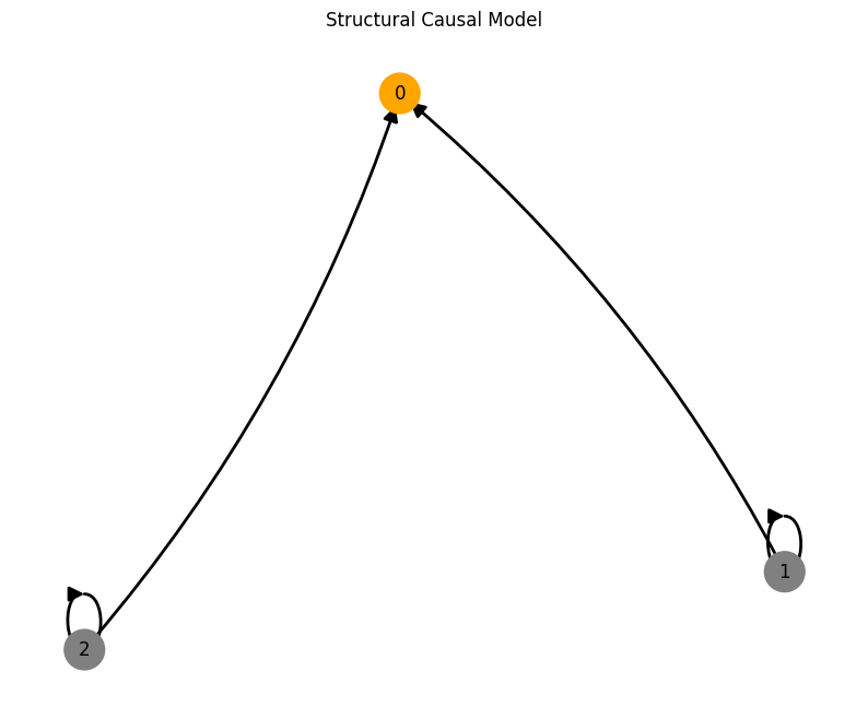
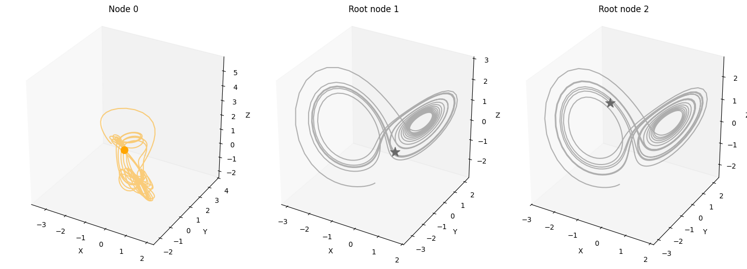
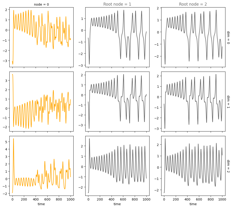
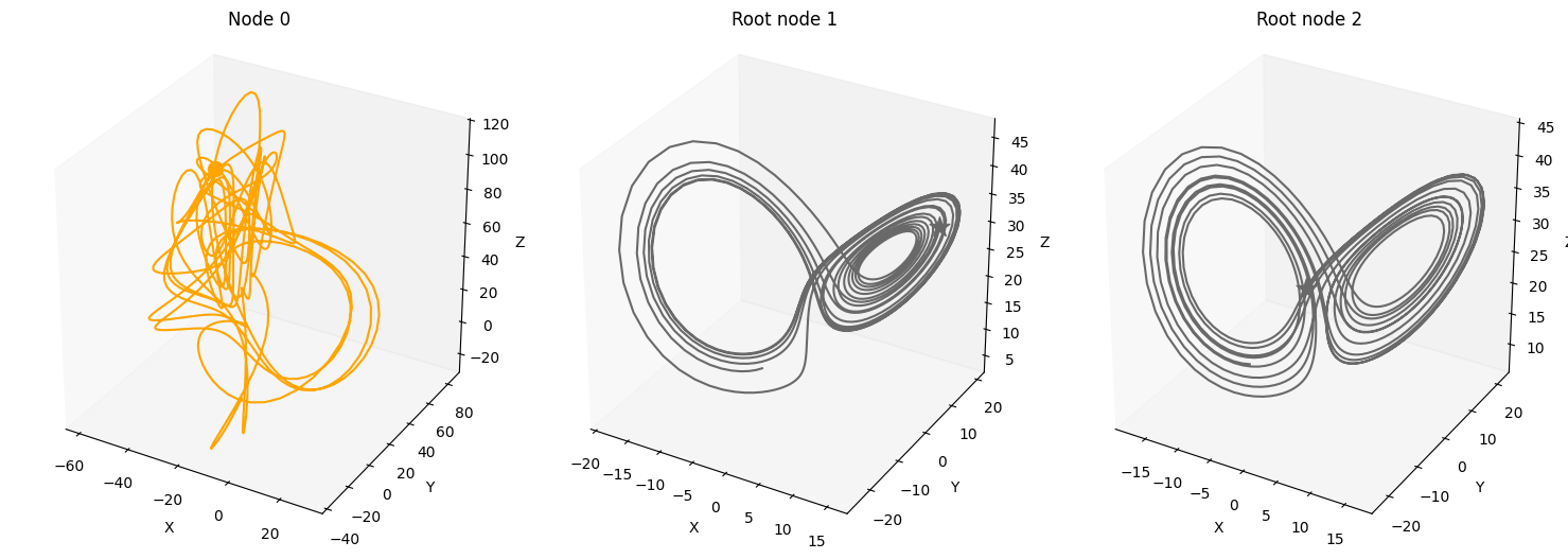
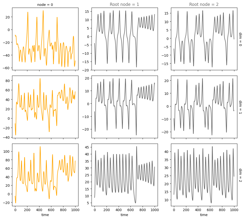
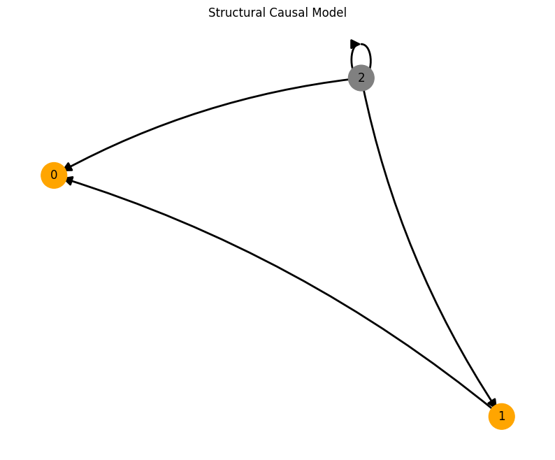
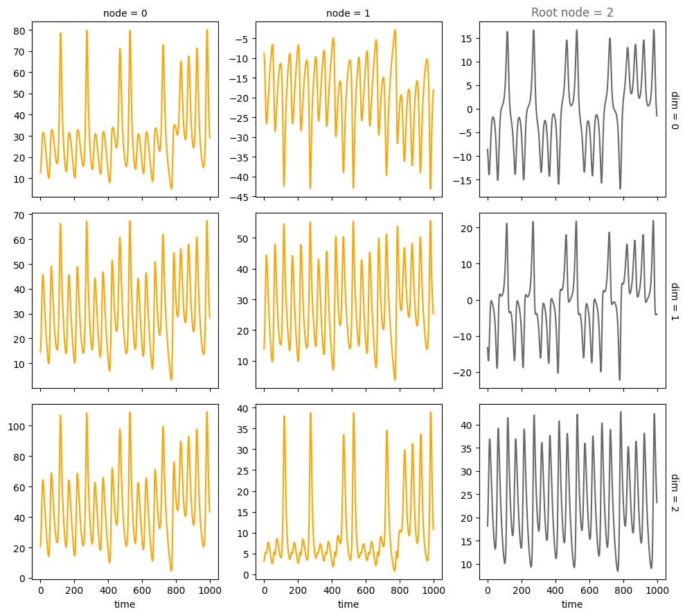
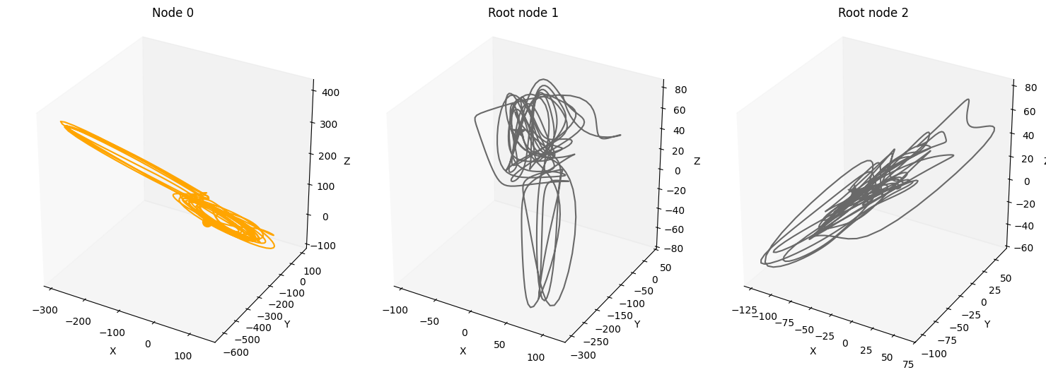
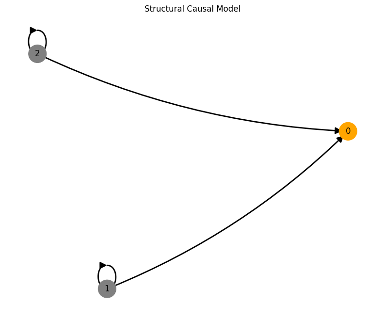
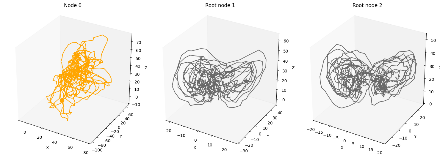
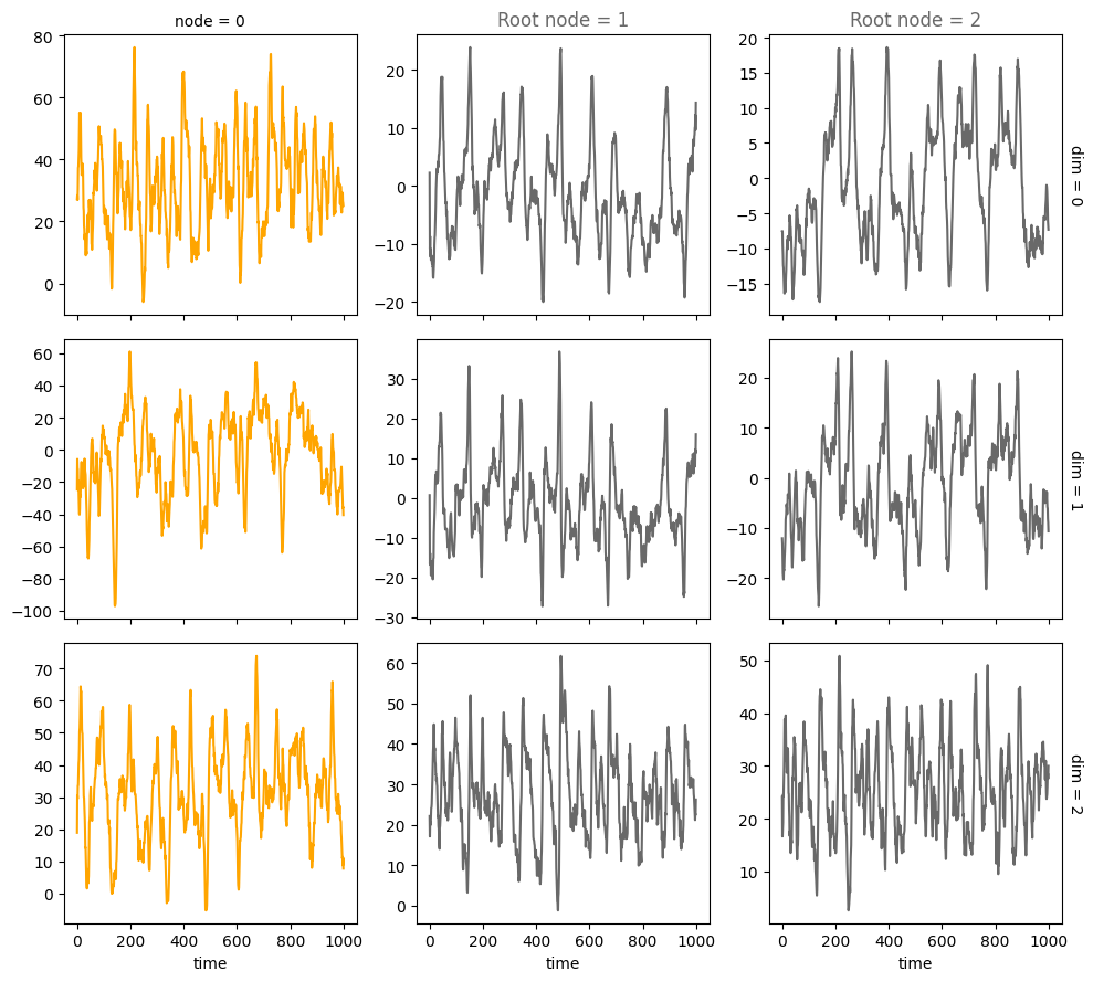
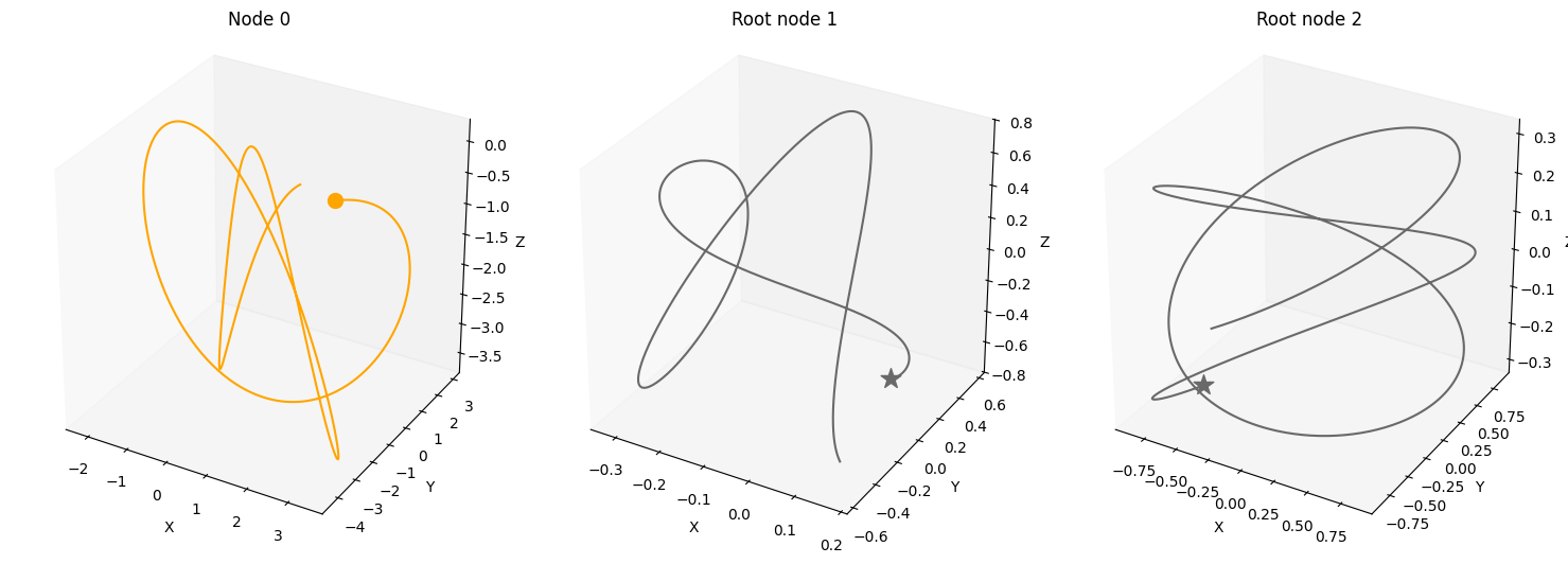
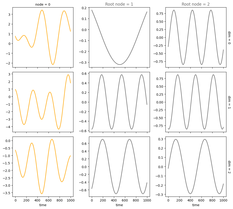
Basic coupled model

num_nodes = 3
node_dim = 3
num_timesteps = 1000

confounders=False,
system_name='Lorenz'

A = torch.tensor([[0,0,0],
                 [1,0,0],
                 [1,0,0]])

A, W, b, root_nodes, _ = create_scm(num_nodes,
                                    node_dim=node_dim,
                                    confounders=confounders,
                                    adjacency_matrix=A)

data = simulate_system(A, W, b, 
                      num_timesteps=num_timesteps, 
                      num_nodes=num_nodes,
                      system_name=system_name) 


plot_scm(G=create_scm_graph(A), root_nodes=root_nodes)
plot_3d_trajectories(data, root_nodes, line_alpha=1.)
plot_trajectories(data, root_nodes, sharey=False)
plt.show()

INFO - Creating SCM with 3 nodes and 3 dimensions each...
INFO - Simulating Lorenz system for 1000 timesteps...

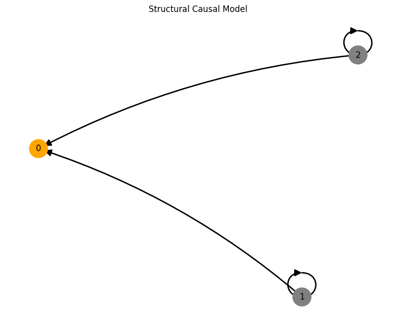
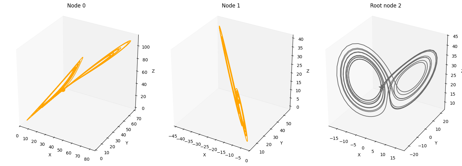
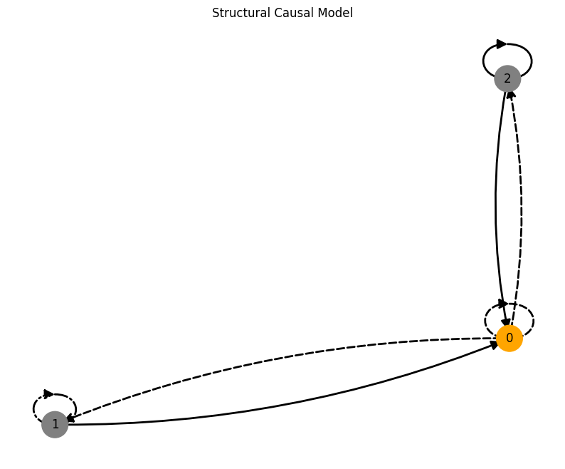
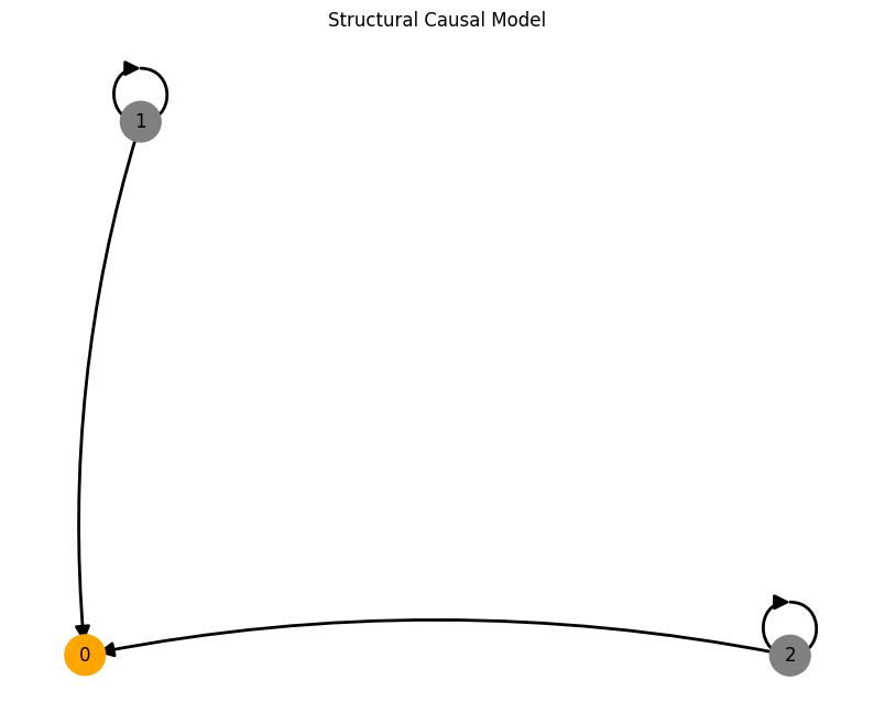
Confounders

A = torch.tensor([[0,0,0],
                 [1,0,0],
                 [1,1,0]])

A, W, b, root_nodes, _ = create_scm(num_nodes,
                                    node_dim=node_dim,
                                    confounders=confounders,
                                    adjacency_matrix=A)

data = simulate_system(A, W, b, 
                      num_timesteps=num_timesteps, 
                      num_nodes=num_nodes,
                      system_name=system_name) 

plot_scm(G=create_scm_graph(A), root_nodes=root_nodes)
plot_3d_trajectories(data, root_nodes, line_alpha=1.)
plot_trajectories(data, root_nodes, sharey=False)
plt.show()

INFO - Creating SCM with 3 nodes and 3 dimensions each...
INFO - Simulating Lorenz system for 1000 timesteps...

Time-lag edges

time_lag = 10
time_lag_edge_probability = 0.1

A, W, b, root_nodes, magnitudes = create_scm(
    num_nodes,
    node_dim=node_dim,
    confounders=False,
    graph="scale-free",
    time_lag=time_lag,
    time_lag_edge_probability=time_lag_edge_probability
)

data = simulate_system(A, W, b, 
                      num_timesteps=num_timesteps, 
                      num_nodes=num_nodes,
                      system_name=system_name,
                      time_lag=time_lag,) 

plot_scm(G=create_scm_graph(A), root_nodes=root_nodes)
plot_3d_trajectories(data, root_nodes, line_alpha=1.)
plot_trajectories(data, root_nodes, sharey=False)
plt.show()

INFO - Creating SCM with 3 nodes and 3 dimensions each...
INFO - Simulating Lorenz system for 1000 timesteps...

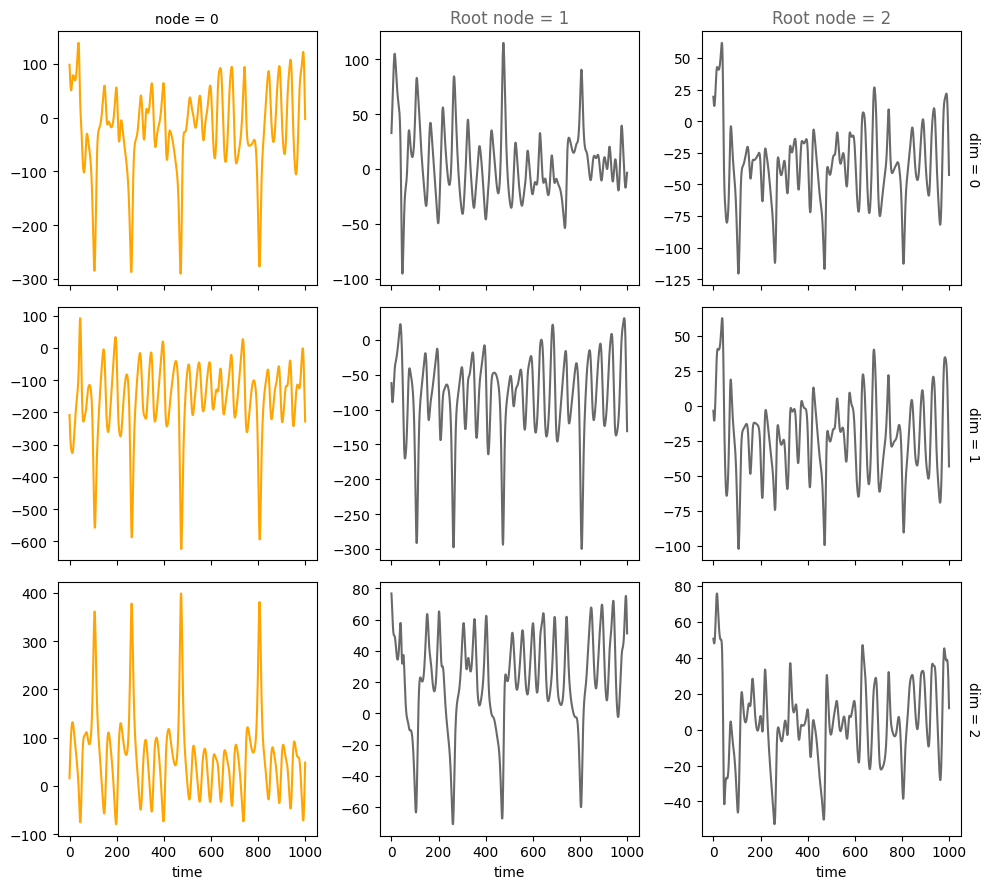
Stochastic systems

num_nodes = 3
node_dim = 3
num_timesteps = 1000
noise = 1.

confounders=False,
system_name='Lorenz'

A = torch.tensor([[0,0,0],
                 [1,0,0],
                 [1,0,0]])

A, W, b, root_nodes, _ = create_scm(num_nodes,
                                    node_dim=node_dim,
                                    confounders=confounders,
                                    adjacency_matrix=A)

data = simulate_system(A, W, b, 
                      num_timesteps=num_timesteps, 
                      num_nodes=num_nodes,
                      system_name=system_name,
                      make_trajectory_kwargs={'noise': noise}) 


plot_scm(G=create_scm_graph(A), root_nodes=root_nodes)
plot_3d_trajectories(data, root_nodes, line_alpha=1.)
plot_trajectories(data, root_nodes, sharey=False)
plt.show()

INFO - Creating SCM with 3 nodes and 3 dimensions each...
INFO - Simulating Lorenz system for 1000 timesteps...

Periodic drivers

num_nodes = 3
node_dim = 3
num_timesteps = 1000

confounders=False,
system_name='Lorenz'

A = torch.tensor([[0,0,0],
                 [1,0,0],
                 [1,0,0]])

A, W, b, root_nodes, _ = create_scm(num_nodes,
                                    node_dim=node_dim,
                                    confounders=confounders,
                                    adjacency_matrix=A)

data = simulate_system(A, W, b, 
                      num_timesteps=num_timesteps, 
                      num_nodes=num_nodes,
                      system_name=system_name,
                      init_ratios=[1,1]) 

plot_scm(G=create_scm_graph(A), root_nodes=root_nodes)
plot_3d_trajectories(data, root_nodes, line_alpha=1.)
plot_trajectories(data, root_nodes, sharey=False)
plt.show()

INFO - Creating SCM with 3 nodes and 3 dimensions each...
INFO - Simulating Lorenz system for 1000 timesteps...

Internal standardization

num_nodes = 3
node_dim = 3
num_timesteps = 1000
standardize = True

confounders=False,
system_name='Lorenz'

A = torch.tensor([[0,0,0],
                 [1,0,0],
                 [1,0,0]])

A, W, b, root_nodes, _ = create_scm(num_nodes,
                                    node_dim=node_dim,
                                    confounders=confounders,
                                    adjacency_matrix=A)

data = simulate_system(A, W, b, 
                      num_timesteps=num_timesteps, 
                      standardize=standardize,
                      num_nodes=num_nodes,
                      system_name=system_name) 


plot_scm(G=create_scm_graph(A), root_nodes=root_nodes)
plot_3d_trajectories(data, root_nodes, line_alpha=0.5)
plot_trajectories(data, root_nodes, sharey=False)
plt.show()

INFO - Creating SCM with 3 nodes and 3 dimensions each...
INFO - Simulating Lorenz system for 1000 timesteps...