Simple causal models

Here, we showcase how to generate data for the simple case, in which we solve single separate dynamical systems such as the Lorenz system. The ODE systems are integrated using the dysts package.

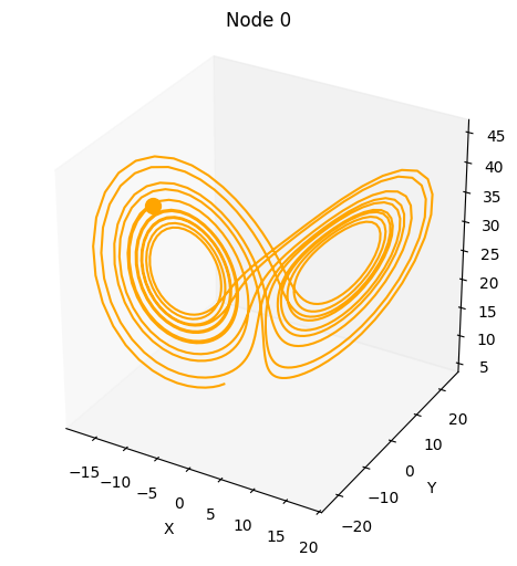
Let’s start by solving a single Lorenz system for 1000 time-steps.

from causaldynamics.systems import solve_system

data = solve_system(num_timesteps=1000, num_systems=1, system_name='Lorenz')
data.shape # [num_timesteps, num_systems, node_dim]

torch.Size([1000, 1, 3])

Let’s visualize the result using the xarray package.

import xarray as xr
import matplotlib.pyplot as plt

from causaldynamics.plot import plot_3d_trajectories

da = xr.DataArray(data, dims=['time', 'node', 'dim'])
plot_3d_trajectories(da)
plt.show()

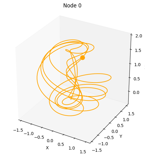
We can also solve a randomly selected dynamical system.

from causaldynamics.systems import solve_random_systems

data = solve_random_systems(num_timesteps=1000, num_systems=1)
da = xr.DataArray(data, dims=['time', 'node', 'dim'])
plot_3d_trajectories(da)
plt.show()

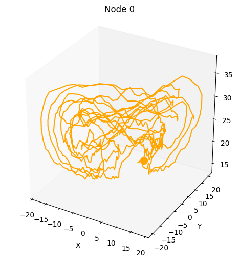
We can also provide kwargs to the underlying dysts.make_trajectory function, e.g. add noise.

from causaldynamics.systems import solve_random_systems

data = solve_random_systems(num_timesteps=1000, num_systems=1, make_trajectory_kwargs={'noise': 0.5})
da = xr.DataArray(data, dims=['time', 'node', 'dim'])
plot_3d_trajectories(da)
plt.show()

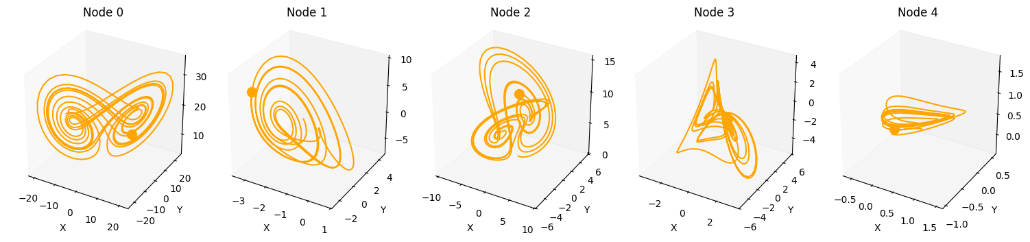
Also, by increasing num_systems we can compute multiple uncoupled dynamical system trajectories in parallel using the same command.

from causaldynamics.systems import solve_random_systems

data = solve_random_systems(num_timesteps=1000, num_systems=5)
da = xr.DataArray(data, dims=['time', 'node', 'dim'])
plot_3d_trajectories(da)
plt.show()