Hierarchically coupled causal models#
Here, we showcase how to generate hierarchically coupled causal models.
import torch
import xarray as xr
import matplotlib as mpl
import matplotlib.pyplot as plt
from causaldynamics.utils import set_rng_seed
from causaldynamics.initialization import initialize_weights, initialize_biases, initialize_x
from causaldynamics.scm import create_scm_graph, get_root_nodes_mask, GrowingNetworkWithRedirection
from causaldynamics.mlp import propagate_mlp
from causaldynamics.systems import solve_system
from causaldynamics.plot import plot_trajectories, animate_3d_trajectories, plot_scm, plot_3d_trajectories
# Set a fixed seed for reproducibility
set_rng_seed(42)
Generate data – the convenient way#
This is the convenient way of generating data. If you need more flexibility, look at the step by step guide below.
This code will first create a coupled structural causal model. The create_scm function returns the adjacency matrix A of the SCM, the weights W and biasses b of all the MLPs located on the nodes and the root_nodes that act as temporal system driving functions.
We use this SCM to simulate a system constisting of num_nodes for num_timesteps and driven by the dynamical systems system_name that are located on the root nodes.
At least, we visualize the results.
from causaldynamics.creator import create_scm, simulate_system, create_plots
num_nodes = 2
node_dim = 3
num_timesteps = 1000
system_name='Lorenz'
confounders = False
A, W, b, root_nodes, _ = create_scm(num_nodes, node_dim, confounders=confounders)
data = simulate_system(A, W, b,
num_timesteps=num_timesteps,
num_nodes=num_nodes,
system_name=system_name)
create_plots(
data,
A,
root_nodes=root_nodes,
out_dir='.',
show_plot=True,
save_plot=False,
return_html_anim=True,
create_animation=False,
)
INFO - Creating SCM with 2 nodes and 3 dimensions each...
INFO - Simulating Lorenz system for 1000 timesteps...
INFO - Generating visualizations
We provide several features that can be used conveniently accessed through the create_scm and simulate_system functions:
from causaldynamics.creator import create_scm, simulate_system
from causaldynamics.plot import plot_scm, plot_trajectories, plot_3d_trajectories
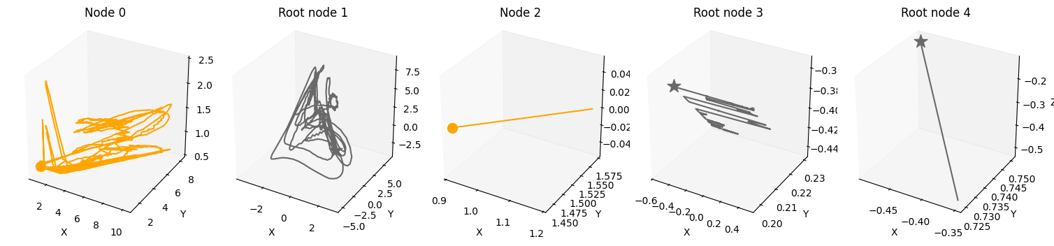
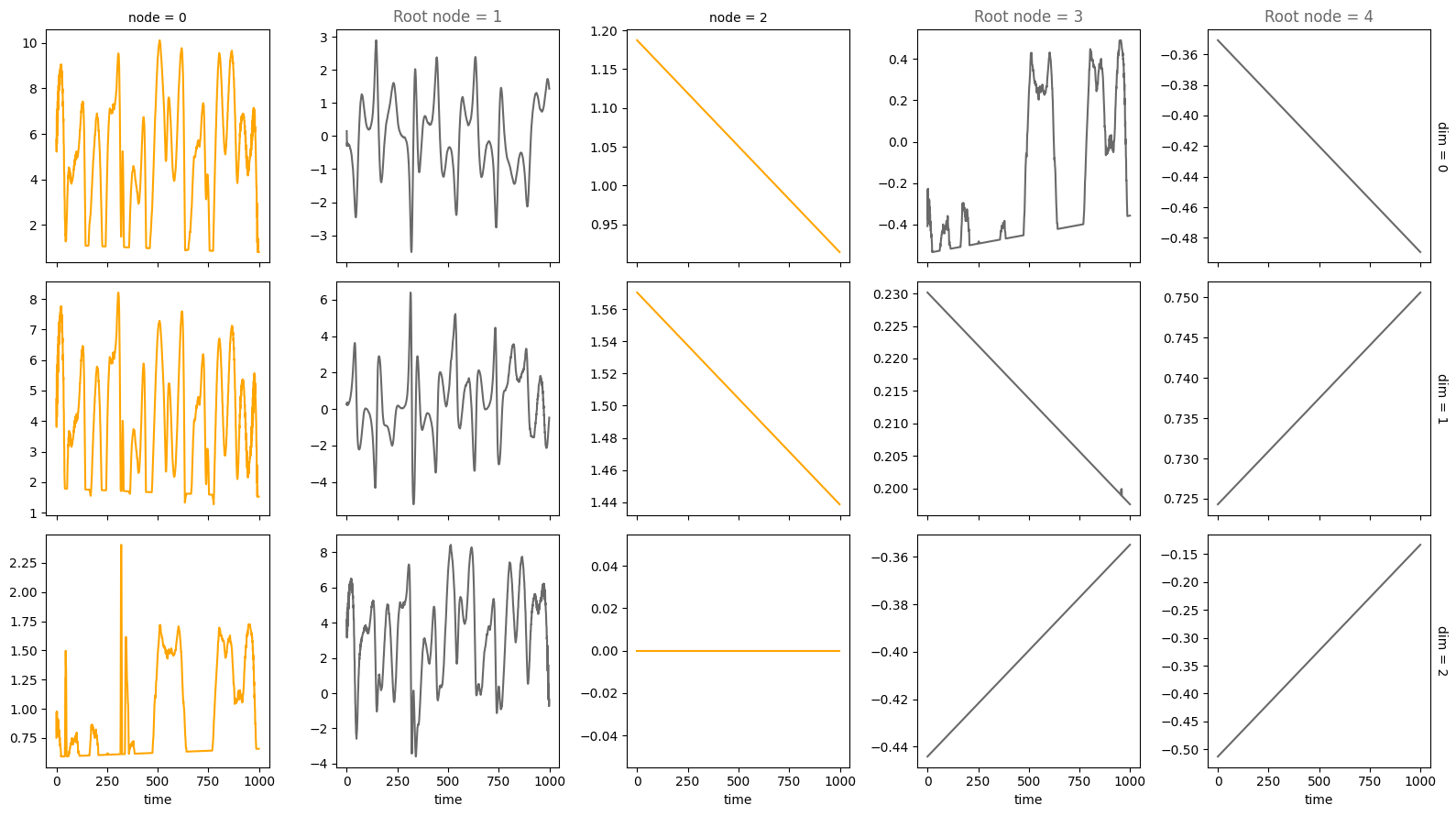
num_nodes = 5
node_dim = 3
num_timesteps = 1000
confounders = False # set to True to add scale-free confounders
standardize = False # set to True to standardize the data
init_ratios = [1, 1, 1] # set ratios of dynamical systems, periodic and linear drivers at root nodes. Here: equal ratio.
system_name='random' # sample random dynamical system for the root nodes
activations_names = ['identity', 'sin', 'sigmoid', 'tanh', 'relu']
noise = 0.5 # set noise for the dynamical systems
time_lag = 10 # set time lag for time-lagged edges
time_lag_edge_probability = 0.1 # set probability of time-lagged edges
A, W, b, root_nodes, _ = create_scm(num_nodes,
node_dim,
confounders=confounders,
time_lag=time_lag,
time_lag_edge_probability=time_lag_edge_probability)
data = simulate_system(A, W, b,
num_timesteps=num_timesteps,
num_nodes=num_nodes,
system_name=system_name,
init_ratios=init_ratios,
time_lag=time_lag,
standardize=standardize,
activations_names=activations_names,
make_trajectory_kwargs={'noise': noise})
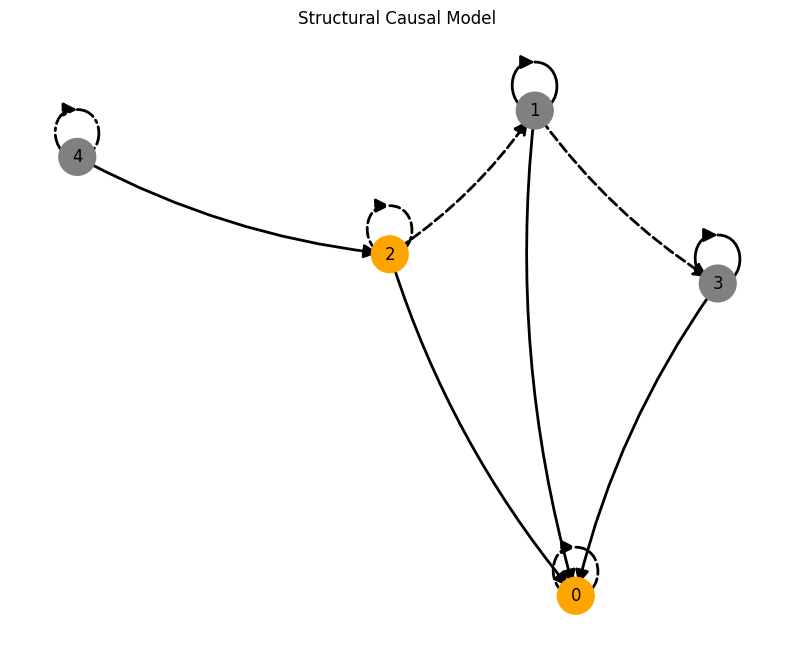
plot_scm(G=create_scm_graph(A), root_nodes=root_nodes)
plot_3d_trajectories(data, root_nodes, line_alpha=1.)
plot_trajectories(data, root_nodes=root_nodes, sharey=False)
plt.show()
INFO - Creating SCM with 5 nodes and 3 dimensions each...
INFO - Simulating random system for 1000 timesteps...
/Users/herdeanu/kausable/causaldynamics/.venv/lib/python3.10/site-packages/dysts/base.py:353: UserWarning: This system has at least one unbounded variable, which has been mapped to a bounded domain. Pass argument postprocess=False in order to generate trajectories from the raw system.
warnings.warn(
For an overview of the features, have a look at the feature.ipynb notebook. If you want more information on specific features, look at their respective notebook, e.g., driver.ipynb or time_lag.ipynb.
Detailed step by step explanation#
Let’s look step-by-step what happens internally in the create_scm and simulate_system functions.
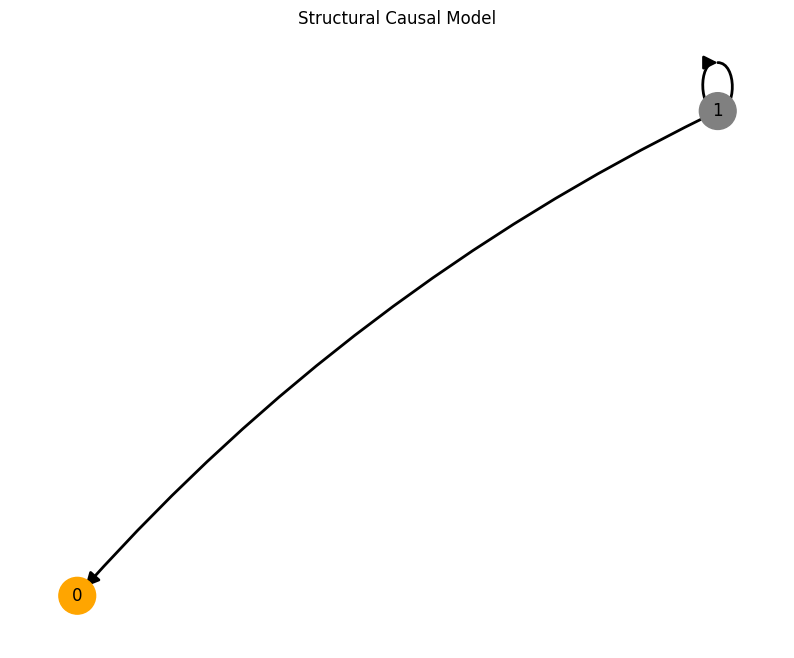
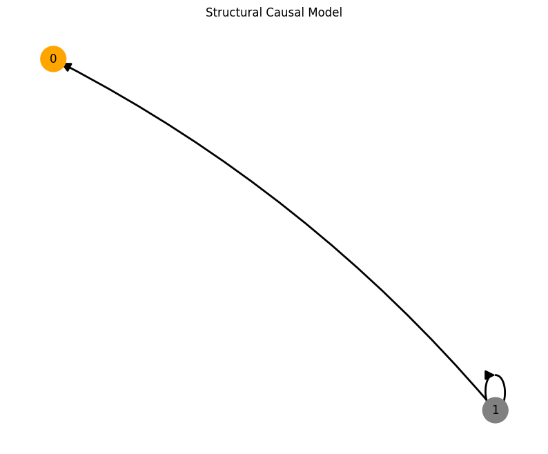
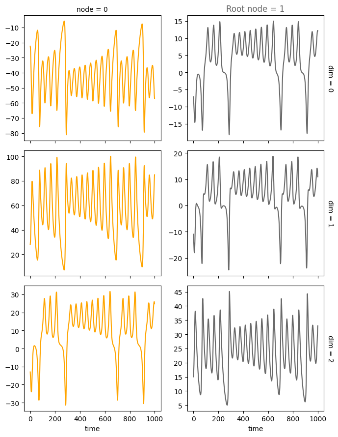
Let’s create a minimal example with a causal graph that has two nodes 0 and 1 and a single edge 1<-0. The signal we send through that graph is given by a Lorenz attractor with dimension 3 that is calculated for some time steps.
# Define parameters for a small test example
N_nodes = 2
N_timesteps = 1000
N_dimensions = 3
# Generate Lorenz attractor trajectory
d_lorenz = solve_system(N_timesteps, N_nodes, "Lorenz")
# Sample the simplest possible adjacency matrix: 0<--1
A = GrowingNetworkWithRedirection(N_nodes).generate()
A
tensor([[0., 0.],
[1., 0.]])
# Sample random weights for the MLPs
W = initialize_weights(N_nodes, N_dimensions)
W
tensor([[[-0.9689, -0.2004, 0.4458],
[ 0.0536, -0.5879, 0.5873],
[ 0.7656, -0.6926, -0.0353]],
[[ 0.4011, -0.5060, -1.7404],
[ 0.7049, 0.0084, 2.3936],
[ 1.2196, 0.5888, 0.0779]]])
# Sample random biases for the MLPs
b = initialize_biases(N_nodes, N_dimensions)
b
tensor([[ 1.1271, -0.4235, -1.7553],
[ 0.9929, -2.5781, 1.0332]])
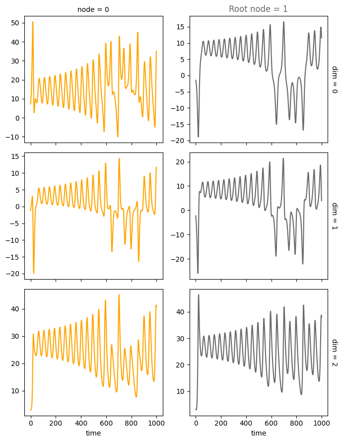
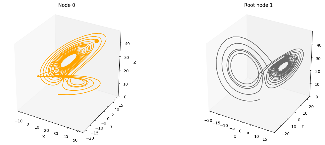
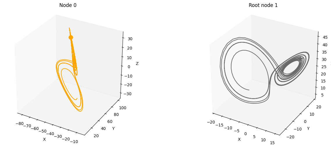
Let’s plot the minimal test graph 1<–0 and propagate the Lorenz attractor through the causal graph.
First, nitialize the root node 1 with the time-series data from the Lorenz attractor. Then, propagate this signal through the edge 1->0. The signal is the input to the sampled multilayer perceptron (MLP) with no activation function. The output is the state of node 0.
# Initialize the root nodes with the Lorenz attractor
init = initialize_x(d_lorenz, A)
# Propagate Lorenz trajectory through the SCM
x = propagate_mlp(A, W, b, init=init)
# Visualize the results using xarray
data = xr.DataArray(x, dims=['time', 'node', "dim"])
root_nodes = get_root_nodes_mask(A)
plot_scm(G=create_scm_graph(A), root_nodes=root_nodes)
plot_3d_trajectories(data, root_nodes, line_alpha=1.)
plot_trajectories(data, root_nodes=root_nodes, sharey=False)
plt.show()
We can even visualize the time unfolding of the system by creating animations. However, this may take a while to run.
# Create an animation of the simple coupled Lorenz attractor.
# Increase the animation limit to 50MB
mpl.rcParams['animation.embed_limit'] = 50 * 1024**2
da_sel = data.isel(time=slice(0, 500))
anim = animate_3d_trajectories(da_sel, frame_skip=2, rotate=True , show_history=True, plot_type='subplots', root_nodes=root_nodes)
display(anim)
INFO - Animation.save using <class 'matplotlib.animation.HTMLWriter'>