Quickstart

0. Installation

Look at the README for installation instructions.

1. Generate data

1.1 Simple causal models

Let’s first look at how to generate data for single dynamical systems. For this, we look at a Lorenz system and solve it for 1000 time steps. Under the hood, the ODE systems are integrated using the dysts package.

Let’s generate the data and visualize the trajectory.

import xarray as xr
from causaldynamics.systems import solve_system
from causaldynamics.plot import plot_3d_trajectories

data = solve_system(num_timesteps=1000, num_systems=1, system_name='Lorenz')
data = xr.DataArray(data, dims=['time', 'node', 'dim'])
plot_3d_trajectories(data)

(<Axes3D: title={'center': 'Node 0'}, xlabel='X', ylabel='Y', zlabel='Z'>,)

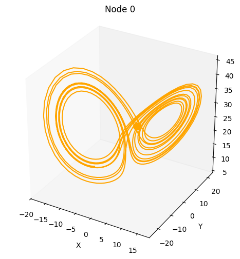
We call the system dimension node for consistency because these systems will later be the driver root nodes in the SCMs.

You can also solve a randomly selected system, pass kwargs to dysts underlying make_trajectory function, or solve multiple dynamical systems in parallel.

For more information, please checkout the more detailed introduction of simple causal models.

1.1 Coupled causal models

Let’s look at how to generate data for the coupled causal models case and visualize it.

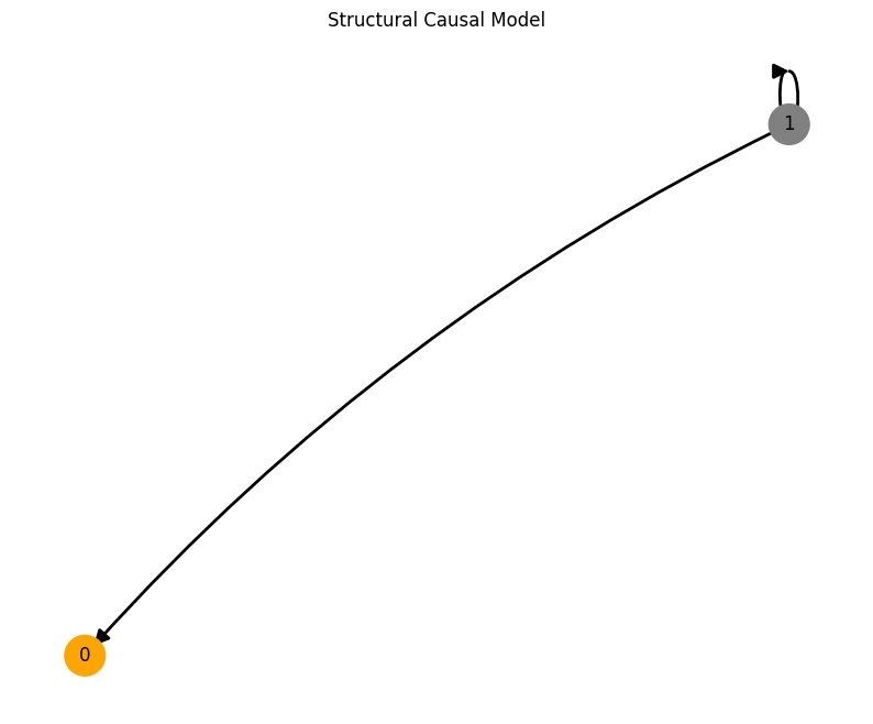
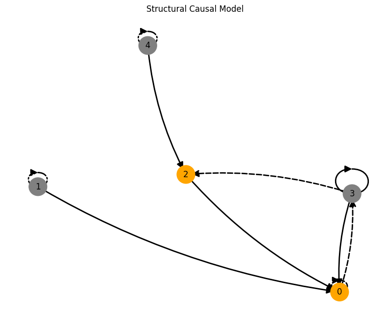
This code will first create a structural causal model. The create_scm function returns the adjacency matrix A of the SCM, the weights W and biases b of all the MLPs located on the nodes and the root_nodes that act as temporal system driving functions.

We use this SCM to simulate a system consisting of num_nodes for num_timesteps and driven by the dynamical systems system_name that are located on the root nodes.

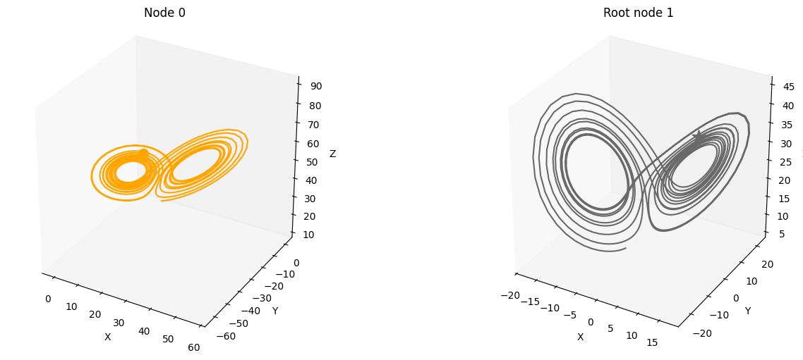
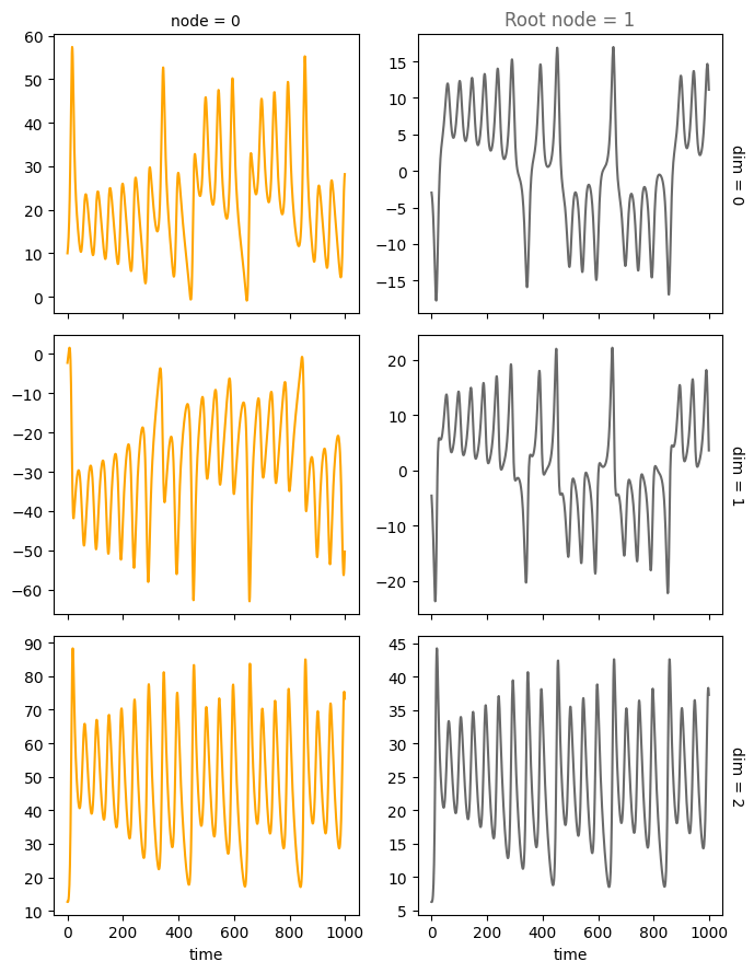
You can get an intuitive understanding of how signals are processed through the edges of the SCM if you take a look at the generated images below. Here, the driving signal from root node 1 is linearly transformed through the MLP on the edge resulting in the signal on node 0.

from causaldynamics.scm import create_scm_graph
from causaldynamics.creator import create_scm, simulate_system
from causaldynamics.plot import plot_scm, plot_trajectories, plot_3d_trajectories

# Define parameters
num_nodes = 2
node_dim = 3
num_timesteps = 1000

system_name='Lorenz'
confounders = False

# Create the coupled structural causal model
A, W, b, root_nodes, _ = create_scm(num_nodes, node_dim, confounders=confounders)

# Simulate the system
data = simulate_system(A, W, b, 
                      num_timesteps=num_timesteps, 
                      num_nodes=num_nodes,
                      system_name=system_name) 

# Visualize the SCM and the system
plot_scm(G=create_scm_graph(A), root_nodes=root_nodes)
plot_3d_trajectories(data, root_nodes)
plot_trajectories(data, root_nodes=root_nodes, sharey=False)

INFO - Creating SCM with 2 nodes and 3 dimensions each...
INFO - Simulating Lorenz system for 1000 timesteps...

<xarray.plot.facetgrid.FacetGrid at 0x3362264a0>

We provide several features that can be conveniently accessed through the create_scm and simulate_system functions:

from causaldynamics.creator import create_scm, simulate_system
from causaldynamics.plot import plot_scm, plot_trajectories, plot_3d_trajectories

num_nodes = 5
node_dim = 3
num_timesteps = 500

confounders = False    # set to True to add scale-free confounders
standardize = False    # set to True to standardize the data
init_ratios = [1, 1]   # set ratios of dynamical systems and periodic drivers at root nodes. Here: equal ratio.
system_name='random'   # sample random dynamical system for the root nodes
noise = 0.5            # set noise for the dynamical systems

time_lag = 10                   # set time lag for time-lagged edges
time_lag_edge_probability = 0.1 # set probability of time-lagged edges


A, W, b, root_nodes, _ = create_scm(num_nodes, 
                                    node_dim,
                                    confounders=confounders,
                                    time_lag=time_lag,
                                    time_lag_edge_probability=time_lag_edge_probability)

data = simulate_system(A, W, b, 
                      num_timesteps=num_timesteps, 
                      num_nodes=num_nodes,
                      system_name=system_name,
                      init_ratios=init_ratios,
                      time_lag=time_lag,
                      standardize=standardize,
                      make_trajectory_kwargs={'noise': noise}) 

plot_scm(G=create_scm_graph(A), root_nodes=root_nodes)
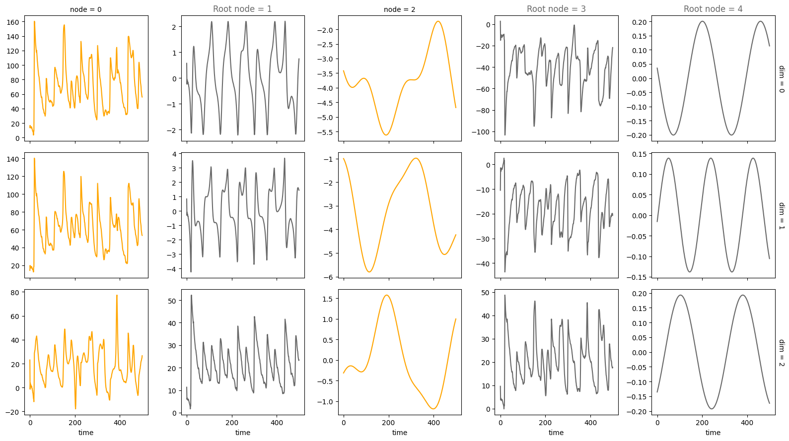
plot_trajectories(data, root_nodes=root_nodes, sharey=False)
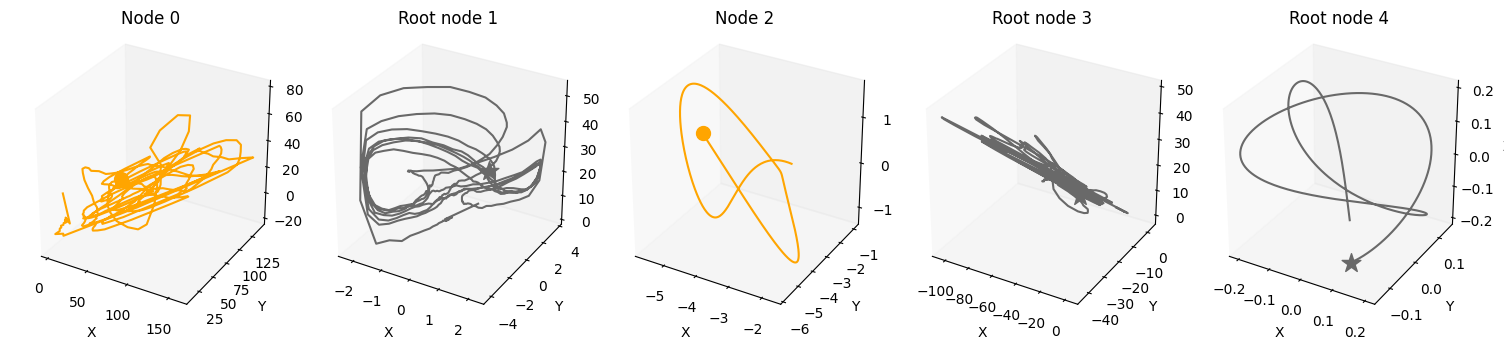
plot_3d_trajectories(data, root_nodes, line_alpha=1.)

INFO - Creating SCM with 5 nodes and 3 dimensions each...
INFO - Simulating random system for 500 timesteps...

(<Axes3D: title={'center': 'Node 0'}, xlabel='X', ylabel='Y', zlabel='Z'>,
 <Axes3D: title={'center': 'Root node 1'}, xlabel='X', ylabel='Y', zlabel='Z'>,
 <Axes3D: title={'center': 'Node 2'}, xlabel='X', ylabel='Y', zlabel='Z'>,
 <Axes3D: title={'center': 'Root node 3'}, xlabel='X', ylabel='Y', zlabel='Z'>,
 <Axes3D: title={'center': 'Root node 4'}, xlabel='X', ylabel='Y', zlabel='Z'>)

For an overview of the features, have a look at the features and the coupled causal models notebook. If you want more information on specific features, look at their respective notebook, e.g., driver, time_lag or standardization.

2. Scripts

We provide several ready to use scripts to generate benchmark data for the simple, coupled, and climate scenario respectively. Have a look at the scripts README.